We can view the world as an 'environment', where for each period an agent is in a state and takes one of the actions available in that state; depending on the configuration of the environment, the agent receives a reward and reaches the next state. In turn, we say that a policy is a vector of probabilities, such that for each state, this vector determines the probability of taking each of the available actions. An environment configured together with a given policy is what is formally known in the RL literature as a Markov Reward Process (MRP).
The objective is going to be to establish how much is the value of following that given policy, from a trajectory of dependent observations (this is framed as an MRP). It may be the case that these observations are generated with the same policy being evaluated or that they are generated with a different policy; in the first case, we will be in an on-policy scenario while in the second we refer to an off-policy scenario (Ramprasad et al, 2022).
Knowing the value of a policy allows us to compare different policies and choose one over the other. A simple example to see this is the case of quarantines, social welfare, and COVID-19; quarantining would allow for greater control of contagion, but at the same time increases poverty levels as people's income-generating capacity is reduced. Suppose you are a ruler and you must decide for each of the 365 days of the year, whether or not to quarantine that day, one policy might be to quarantine only on even days, another policy might be to quarantine every 3 months, and so on. These are part of the range of policies you can implement, you want to compare them and based on that decide which one to implement.
Now, finding the value function of a policy is not trivial; in the best case, you know all the information about the environment and you can easily access it, when this happens, the Bellman equation allows you to find the value function without much effort (Sutton & Barto, 2018). However, it is common that in RL there is uncertainty or the environment is very large, and therefore we cannot use this equation.
In these cases, RL can use alternatives, one of them being Linear Stochastic Approximation (LSA). This is an iterative algorithm that allows finding solutions to linear equations starting from observed data with uncertainties (Haskell, 2018). In the general framework, the LSA error is a martingale difference, in simple words, it is to relax the independence assumption and that the error has "zero mean" so that the LSA algorithm converges. The problem is that when LSA is applied to RL, using a linear approximation of the value function, this assumption is violated and the noise becomes Markovian, referring to the fact that now the noise depends on a discrete stochastic process such that the probability of occurrence of an event depends on the immediately preceding event.
Still, Liang (2010) shows that it is theoretically possible to write the Markovian noise as a martingale noise and another part of decreasing residual noises. Although this allows us to continue applying LSA; in practice, it is not possible to obtain these values separately, so the results will be biased. Among the classical LSA methods applied to RL are Time Differences (TD) for the on-policy case, while for the off-policy case, they are the Gradient of Time Differences (GTD) methods. These methods, while performing quite acceptably, can be improved by trying to correct for the bias mentioned above.

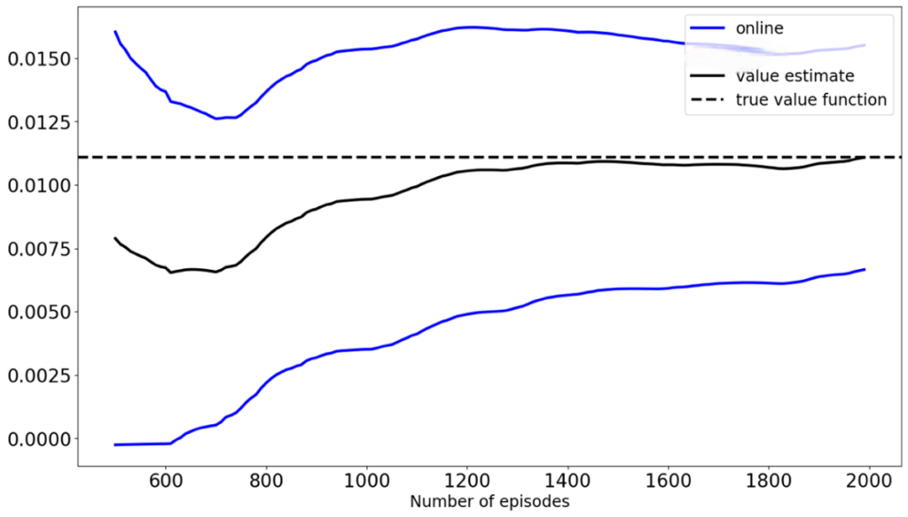
Figure 1: TD vs. the Online Bootstrap.
Precisely to make this improvement, Ramprasad et al (2022) propose the Online Bootstrap Inference method. This consists of adding a statistical bootstrap to the classical methods, where for each period B penalized iterations of the LSA parameter are performed and from this, confidence intervals for the value function are constructed. Graph 1 shows a comparison between TD and the Online Bootstrap for the Frozen Lake environment of OpenAI gym, and an epsilon-greedy policy with e=0.2. This is constructed with the code proposed by Ramprasad et al (2022). The results show that TD (black line) closely approximates the true value of the value function (dashed line) although it has a mistake up to 2000 iterations, while the Online Bootstrap (blue lines) guarantees that the true value function will be within the confidence interval from 600 iterations onwards. On the other hand, we found that as the randomness of the policy to be evaluated increases, the convergence of the Online Bootstrap algorithm slowed down and the width of the confidence intervals increased significantly.
References:
Haskell, W. B. (2018). Introduction to dynamic programming. Na- tional University of Singapore. ISE 6509: Theory and Algorithms for Dynamic Programming.
Liang, F. (2010). Trajectory averaging for stochastic approximation mcmc algorithms. The Annals of Statistics.Vol. 38, No. 5 (October 2010), pp. 2823- 2856.
Ramprasad, P., Li, Y., Yang, Z., Wang, Z., Sun, W., and Cheng, G. (2022). Online bootrstrap inference for policy evaluation in reinfor- cement learning. Journal of the American Statistical Association, pp. 1-14.
Sutton, R. and Barto, A. (2018). Reinforcement learning: An introduction. The MIT Press.
Get information about Data Science, Artificial Intelligence, Machine Learning and more.
In the Blog articles, you will find the latest news, publications, studies and articles of current interest.