
Looking at the Distribution, Not Just the Average
Suppose a government implements a new health policy aimed at reducing avoidable hospitalizations. A traditional evaluation might tell us that, on average, hospitalizations fall by 10%. But that single figure hides key questions: Who benefits the most—high-risk patients or medium-risk patients? Does the policy reduce extreme events (colas of the distribution) or only improve moderate situations? Is the impact similar across different regions or adoption cohorts?
Quantile Regression (QR) addresses precisely these kinds of questions. Instead of focusing on the conditional mean of an outcome Y given X, it allows us to study how a given quantile (for example, the 25th, 50th, or 75th percentile) changes when a policy is introduced. Schematically, quantile regression estimates, for a given percentile, a linear predictor that approximates the conditional quantile. Instead of penalizing errors quadratically (as OLS does), QR uses a loss function that penalizes positive and negative residuals differently, so that the percentile is properly centered.
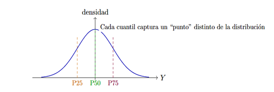
Figure 1: Quantile regression: looking at how each quantile of the distribution shifts, not just the average.
In the evaluation of policies implemented in a staggered manner over time (where implementation is not simultaneous for all beneficiaries), it is natural to combine QR with difference-in-differences (DiD) designs. The question is: can we simply use a quantile regression with two-way fixed effects (TWFE-QR) and feel confident about the results?
Our work shows that the answer is no, and that the problem of forbidden comparisons, already known in the context of means, carries over—subtly—to quantiles.
The Scenario: Policies with Staggered Adoption
Imagine a panel with units i (municipalities, hospitals, firms) and periods t (years, quarters, months). Each unit adopts a policy at a different point in time: some early, others late, and some never. The TWFE-QR estimator seeks the value that best fits the quantiles of the outcome variable’s distribution once fixed effects have been absorbed. At first glance, this is a natural extension of classical TWFE to the world of quantiles. However, when adoption is staggered and policy effects differ across cohorts, the TWFE-QR estimator ends up mixing treated-versus-treated comparisons across different periods, something that goes against the logic of the DiD design.
What TWFE-QR Is Actually Doing
Behind the scenes, quantile regression with fixed effects solves a convex optimization problem. The Karush–Kuhn–Tucker (KKT) conditions impose that, at the optimum, certain residual balances must equal zero when weighted by the covariates (including the treatment variable). Without going into the technical notation, the key message is that for each cohort g (defined by the timing of adoption) and period l, we can think of a score associated with the cell (g,l): it measures how many observations lie above or below the target quantile. The TWFE-QR estimator chooses a single value for the treatment effect estimator such that the sum of all these scores, aggregated across all treated cells, balances out to zero. If every cohort had the same policy effect, this balance would be coherent: all cells would “push” in the same direction. But when effects differ across cohorts (heterogeneity), some cells push upward, others downward, and the final result becomes a kind of weighted average of cohort effects.
In our work, we show that under fairly general conditions, TWFE-QR can be interpreted as a weighted average of the “clean” effects of each cohort g (if it were compared only against appropriate controls), with nonnegative weights that depend on cohort size, the number of treated periods, and how informative the distribution is around the quantile of interest. The problem is that these weights do not explicitly follow a policy logic, but instead emerge from the KKT conditions. The weights depend on the structure of the panel and on the density of the distribution around the quantile of interest, not on an explicit design criterion. From a public policy perspective, this complicates interpretation: what effect are we actually reporting? Does it correspond to a treated-versus-never-treated contrast, or does it mix treated-versus-treated comparisons across different stages of adoption?
Our Proposal
To address this problem, we propose an alternative estimator based on a simple idea: we construct clean cohort-specific contrasts and then aggregate them using weights with a clear interpretation. The procedure is as follows:
The key is that each 2×2 comparison effect is constructed while avoiding treated-versus-treated comparisons at inappropriate times, and that the final aggregation respects the design logic: more weight is assigned to cohorts with a larger number of treated observations, but without allowing treated units to serve as their own controls at another stage.
What We Found in Simulations
To illustrate the behavior of both estimators, we consider a simulated data experiment in which: the untreated outcome combines a unit fixed effect, a time fixed effect, and a random shock; and the policy effect is heterogeneous across cohorts—some cohorts have a larger impact in the upper tail, others around the median, and so on. In this setting, we compare: the aggregated TWFE-QR estimator, which estimates a single effect for the entire panel, and the cohort-based estimator with transparent aggregation. The results show that: TWFE-QR exhibits substantial bias at several quantiles (P25, P50, P75) when effects are heterogeneous. In some scenarios, the sign of the estimated effect does not match the true effect. Our estimator systematically reduces bias across the distribution: the percentage bias falls substantially between P25 and P75, and the estimator preserves the correct direction of the effect at all quantiles.

Figure 2: TWFE: target and bias across percentiles. In simulations with four cohorts (early, middle, late, and never treated), the TWFE-QR estimator exhibits substantial bias and, at some quantiles, can even reverse sign relative to the true effect (orange). Our proposal (green) consistently reduces bias at P25, P50, and P75.
Beyond the numerical metrics, the qualitative interpretation also improves: the analyst can decompose the effect into cohort-specific components, identify which groups benefit the most at each quantile, and communicate results in a way that aligns with the actual structure of the policy (who was treated and when).
Implications
At this stage of our research, the main findings have been the following: if the policy is adopted at different times and there is reason to suspect heterogeneous effects, using TWFE-QR mechanically leads to misleading interpretations: the estimator mixes early and late treatments as if they were controls for one another. At a minimum, a design based on clean cohort-specific comparisons is necessary to preserve the original DiD logic: comparing treated units only with “never treated” or “not yet treated” units, and then constructing an average that reflects that structure. The transparency of the weights is crucial: knowing exactly how much each cohort contributes to the aggregated effect facilitates communication with decision-makers and the design of targeted policies.
Get information about Data Science, Artificial Intelligence, Machine Learning and more.
References
Goodman-Bacon, A. (2021). Difference-in-Differences with Variation in Treatment Timing. Journal of Econometrics, 225(2), 254-277.
Callaway, B., & Sant’Anna, P. H. C. (2021). Difference-in-Differences with Multiple Time Periods. Journal of Econometrics, 225(2), 200-230.
Sun, L., & Abraham, S. (2021). Estimating Dynamic Treatment Effects in Event Studies with Heterogeneous Treatment Effects. Journal of Econometrics, 225(2), 175-199.
In the Blog articles, you will find the latest news, publications, studies and articles of current interest.